You can grasp how satellites and spacecraft move without doing any equations. Orbital mechanics is simply the set of rules that describe how objects fall around a planet or the Sun — how speed, altitude, and direction combine to make stable or changing paths. This article shows those rules with clear examples and everyday analogies so you can visualize orbits, plane changes, transfers, and rendezvous without math.

Expect short, concrete explanations of orbital shapes, why some paths stay fixed while others decay, and what forces — like gravity, drag, and thrust — actually do to a spacecraft. Along the way you’ll see practical uses: launch windows, Geostationary orbits, and why plane changes cost fuel, all explained in plain language that connects concepts to real missions.

What Is Orbital Mechanics?

Orbital mechanics explains how objects travel around each other, how gravity shapes those paths, and how engineers use those principles to place and steer satellites and spacecraft. You’ll learn how motion, forces, and predictable patterns combine to make orbits useful and navigable.

How Objects Move in Space

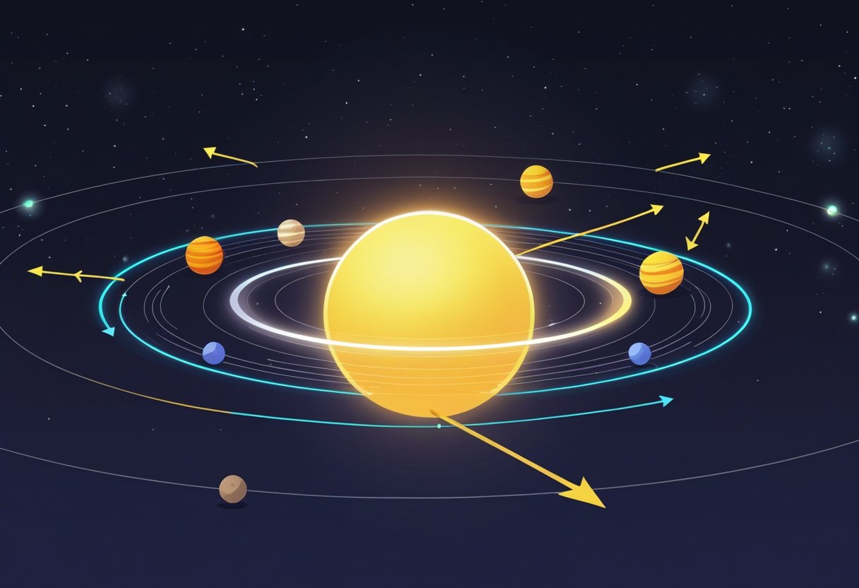
You can think of motion in space as a balance between straight-line travel and a constant pull toward another body. When you launch an object it keeps moving forward, but gravity bends that motion into a curve. If the forward speed matches the curved drop caused by gravity, the object keeps missing the ground and becomes an orbiting body.

Practical terms matter: velocity and altitude determine whether you get a low, fast orbit like many Earth-observing satellites, or a higher, slower orbit such as geostationary satellites. Small effects—atmospheric drag, engine firings, or pulls from other bodies—nudge orbits over time. You monitor and correct those nudges to keep a satellite on task.

The Role of Gravity

Gravity is the central force that creates and sustains orbits. You feel this when you drop something on Earth; in space, the same attraction keeps satellites circling planets and moons circling planets. The strength of gravity depends on mass and distance: heavier bodies and closer distances produce stronger pulls.

You’ll notice gravity also governs orbital energy and stability. A stronger pull at lower altitudes requires higher speed to avoid falling, while weaker pull farther out lets objects orbit more slowly. Interactions among multiple gravitational sources—like the Earth, Moon, and Sun—cause predictable variations called perturbations that operators must manage.

Orbital Motion and Celestial Mechanics

Celestial mechanics provides the rules and history behind orbital motion, tracing from Kepler’s description of planetary paths to modern mission planning. You use those same concepts to predict satellite positions, plan transfers between orbits, and time launches to exploit planetary alignment. The two-body picture (one primary, one satellite) gives clear, useful results for many tasks.

In more complex situations you consider additional forces and bodies. Celestial mechanics supplies tools to handle those: conserved quantities like angular momentum and energy, and approximations that simplify multi-body interactions. Applying those tools helps you predict motion accurately without heavy math, so you can visualize trajectories, design maneuvers, and keep spacecraft where you need them.

Foundations of Orbital Motion

You will learn why planets and satellites follow predictable paths, how motion and gravity connect, and which simple rules let engineers plan maneuvers precisely. Expect clear, concrete ideas: shapes of orbits, how sweep rates link to speed, and why gravity acts at a distance.

Johannes Kepler and His Laws

Kepler identified three practical rules from precise observations of Mars. First, orbits are ellipses with the Sun at one focus—this law of ellipses replaces the older idea of perfect circles. You should picture each orbit as a stretched circle defined by its eccentricity (how elongated it is).

Second, the law of equal areas (Kepler’s second law) says a line from the Sun to a planet sweeps equal areas in equal times. That means you move faster when you are closer to the Sun and slower when you are farther away. This explains why planets speed up near perihelion and slow near aphelion.

Third, Kepler’s third law relates orbital size to period: the square of a planet’s orbital period scales with the cube of its average distance from the Sun. In practice, if you know the semi-major axis, you can predict how long an orbit takes. These laws give you direct, testable relationships without invoking forces.

Isaac Newton’s Revolutionary Ideas

Newton explained why Kepler’s rules work by introducing motion laws you can apply to any moving object. His three laws of motion tell you how velocity changes when forces act: inertia, F = ma, and action–reaction. These let you predict how a spacecraft responds to a rocket burn.

Newton combined these with the idea that the Sun’s pull weakens with distance to derive elliptical orbits from forces. Practically, that means the same mechanics that govern a thrown ball also govern planets. You can treat orbital changes as push-and-response events: apply thrust and the orbit reshapes predictably.

Engineers use Newton’s formulation to compute trajectories, rendezvous burns, and transfer orbits. Newton turned descriptive rules into a predictive toolbox you can use to design a mission or explain why Kepler observed what he did.

The Law of Universal Gravitation

Newton’s law of universal gravitation states that every two masses attract with a force proportional to the product of their masses and inversely proportional to the square of their separation. Concretely, doubling the distance cuts the gravitational pull to one quarter, and doubling either mass doubles the force.

This inverse-square rule explains orbital strength at different altitudes: lower orbits require higher tangential speed to balance stronger gravity. It also defines escape conditions—if you supply enough kinetic energy to overcome gravitational binding, the object will not return.

Use this law together with Newton’s motion laws to derive orbital behaviors such as circular speed, elliptical shape, and transfer maneuvers. In the field, combining specific angular momentum with specific mechanical energy (both conserved without external forces) gives you practical formulas for altitude, speed, and orbital period.

Shapes and Types of Orbits

Orbits differ mainly by shape and by how fast an object moves relative to escape speed. You’ll learn which paths keep a spacecraft bound to a planet, which let it escape, and how a single parameter — eccentricity — classifies them.

Understanding Elliptical and Circular Orbits

A circular orbit is a special case of an ellipse where eccentricity equals zero. In a circular orbit your altitude stays constant and orbital speed remains nearly uniform, which simplifies station-keeping and communications for satellites. Geostationary satellites use circular orbits at a precise radius so they remain fixed above a point on Earth.

Elliptical orbits have eccentricity between 0 and 1. You’ll see varying altitude: the closest point (perigee) gives higher speed, the farthest point (apogee) gives lower speed. That speed change follows conservation of energy and angular momentum, which makes transfer maneuvers like Hohmann transfers efficient when you change altitude at the right orbital point.

Practical uses differ: low, nearly circular orbits suit Earth observation; more eccentric elliptical orbits suit missions needing long dwell time over high latitudes. You can think of circular orbits as a subset of elliptical orbits with simplified behavior.

Parabolic and Hyperbolic Trajectories

Parabolic and hyperbolic paths occur when an object reaches or exceeds escape velocity. A parabolic trajectory corresponds to exactly escape velocity; technically its eccentricity equals 1. If your vehicle follows a parabolic path, it will never return but its excess speed at infinity is effectively zero.

Hyperbolic trajectories have eccentricity greater than 1. In this case your spacecraft has positive hyperbolic excess velocity (v∞) and departs the gravity well on a path whose shape is an open curve. Gravity bends your inbound and outbound paths; the angle of deflection depends on approach speed and closest approach distance. Flybys that alter spacecraft velocity relative to the Sun often use hyperbolic legs to gain or shed orbital energy.

Both parabolic and hyperbolic paths are used in interplanetary mission design: hyperbolic excess velocity and geometry matter for planning launch energy and planetary encounters.

Conic Sections in Orbit

All the main orbital shapes are conic sections: circles and ellipses (closed), parabolas (marginal), and hyperbolas (open). Eccentricity (e) serves as the single classifier: e = 0 (circle), 0 < e < 1 (ellipse), e = 1 (parabola), e > 1 (hyperbola). This single number tells you whether an orbit is bound and how stretched the path is.

Use this quick reference for mental calculations:

• e = 0 → circular orbit, constant radius.
• 0 < e < 1 → elliptical orbit, varying radius (perigee/apogee).
• e = 1 → parabolic trajectory, escape borderline.
• e > 1 → hyperbolic trajectory, unbound escape.

Knowing the conic type helps you predict speed changes, transfer maneuver points, and whether a spacecraft will remain captured by the planet or escape into interplanetary space. For a concise primer on orbital mechanics concepts, see this overview of orbital mechanics fundamentals.

Key Features of Orbits

Orbits have measurable size, shape, orientation, and timing that determine where an object will be and how fast it moves. You will learn what sets orbital speed and period, where closest and farthest points occur, and which orbital elements define the orbit’s geometry and position.

Orbital Period and Orbital Speed

The orbital period tells you how long a satellite takes to complete one revolution around the system’s center of mass. For Earth satellites, period correlates directly with the semi-major axis: larger semi-major axis = longer period. You can use mean motion (revolutions per day) to get the period quickly.

Orbital speed changes along the path for non-circular orbits. You move fastest near periapsis (perigee for Earth, perihelion for the Sun) and slowest near apoapsis (apogee for Earth, aphelion for the Sun). Circular orbits keep a constant orbital speed and single radius, while elliptical orbits trade speed for radial distance.

Practical note: low Earth orbits (small semi-major axis) yield short periods (~90–120 minutes) and high average speeds, while geostationary altitude (large semi-major axis) yields a 24-hour period and much lower orbital speed.

Periapsis, Apoapsis, and Special Points

Periapsis and apoapsis mark the closest and farthest points in an orbit from the center of mass. You will see specific names depending on the central body: perigee/apogee for Earth, perihelion/aphelion for the Sun. These points set the orbit’s radial extremes and control instantaneous speed and atmospheric drag exposure for low orbits.

The argument of periapsis locates periapsis within the orbital plane; the longitude of the ascending node fixes where the orbit crosses the reference plane going north. True anomaly gives the satellite’s angular position measured from periapsis at a specific time. Mean anomaly provides a time-based proxy for position used in propagation, while eccentric anomaly is a geometric angle used to convert mean anomaly into true anomaly.

You should watch periapsis closely for reentry risk or for missions that need close passes. Apoapsis often serves mission needs requiring long dwell times or high-altitude sensing.

Orbital Elements and Their Meaning

Six classical orbital elements describe size, shape, orientation, and position: semi-major axis (a), eccentricity (e), inclination (i), longitude of ascending node (Ω), argument of periapsis (ω), and true anomaly (ν) at epoch. The semi-major axis sets the overall energy and period; eccentricity sets how stretched the orbit is.

Inclination tells you the tilt relative to the reference plane and controls which latitudes you overfly. Ω orients the orbital plane around the central body. ω defines where the closest approach sits inside that plane. The true anomaly (or mean anomaly at epoch) tells you where the object is along the path at the epoch time.

Together these elements let you reconstruct the orbit around the system’s center of mass and predict future positions using propagation methods.

Specific Orbits Around Earth and Beyond

You’ll learn where different satellites live, why each orbit fits certain missions, and how altitude and inclination change a satellite’s behavior.

Low Earth Orbit, GEO, and More

Low Earth Orbit (LEO) sits roughly 160–2,000 km above Earth. You’ll find Earth-observation, crewed stations, and many communication constellations here because LEO gives low latency and high-resolution imaging. Speeds are high — about 7.8 km/s near 300 km — so satellites complete orbits in ~90–120 minutes.

Geosynchronous and geostationary orbits (GEO) are near 35,786 km altitude. A geostationary satellite stays fixed over one longitude on the equator, making it ideal for continuous TV, weather monitoring, and regional communications. Geosynchronous but inclined orbits repeat ground tracks daily but appear to oscillate north–south.

Transfer orbits like Geostationary Transfer Orbit (GTO) bridge LEO and GEO. You launch into an elliptical GTO, then use a burn at apogee to circularize at GEO. That saves fuel versus a direct ascent.

Unique Orbits for Different Missions

You choose orbit shape and inclination to meet mission needs. Molniya orbits are highly elliptical with long dwell time over high latitudes; you’d use them for communications in northern regions where GEO can’t provide good coverage. Interplanetary missions use escape trajectories, not bound Earth orbits, to reach other planets.

Mission planners balance coverage, revisit time, and lifetime. For continuous global broadband you might deploy thousands of small LEO satellites in coordinated planes. For persistent imaging of a city, lower LEO altitudes and sun-synchronous timing increase resolution and consistent lighting. Each choice changes propulsion, launch profile, and collision risk.

Polar and Sun-Synchronous Orbits

Polar orbits pass over or near both poles every revolution, so your satellite can eventually see the entire globe as Earth rotates beneath it. These orbits suit mapping, reconnaissance, and polar science where global coverage matters.

Sun-synchronous orbits (SSO) are a special polar family that keeps a constant local solar time at each ground pass. You’ll use SSO for consistent shadows and illumination in imaging and remote sensing. Typical altitudes range 600–800 km with inclinations near 98°, and the orbital plane precesses to track the Sun. SSO makes comparing images over time much simpler for monitoring land use, crops, or ice.

How Orbits Change and What Affects Them

Orbits change when you alter a spacecraft’s speed, direction, or the forces acting on it. Small, well-timed burns and external influences like atmosphere or third-body gravity produce large effects on where and when you arrive.

Orbital Transfers and Maneuvers

You change orbit by changing your velocity (delta‑V). The most common planned method is the Hohmann transfer, which uses two burns: one to raise apoapsis and one to circularize at the new altitude. A Hohmann transfer orbit is fuel-efficient for moving between two coplanar circular orbits when time is not critical.
If you must change inclination as well as altitude, combining a plane change with a tangential burn at apoapsis lowers delta‑V cost. For larger or faster changes, you may use multiple burns, bi‑elliptic transfers, or continuous low‑thrust spirals from electric propulsion.
Phasing maneuvers time your arrival for rendezvous, and launch windows control when you can reach a given orbital plane from the ground. Plan your burns around points of lowest velocity (apogee) for the cheapest plane changes.

Escape Velocity and Gravity Assists

Escape velocity is the speed you need to stop being bound to a planet; reach it and your trajectory becomes an open path rather than a closed orbit. If you exceed escape velocity by just a little, you carry residual speed (hyperbolic excess) useful for interplanetary travel.
Gravity assists let you change speed and direction without burning propellant. You fly close to a planet and exchange momentum: the planet’s motion boosts (or reduces) your heliocentric velocity. Gravity assists shape many interplanetary trajectories and can cut fuel needs dramatically, but they fix timing and geometry—your launch window must align with planetary positions.
Use gravity assists for missions where you need extra energy for deep-space targets or to alter inclination cheaply.

Non-Ideal Factors: Drag and Perturbations

Atmospheric drag slowly lowers low‑Earth orbits by removing energy each pass; you correct it with periodic reboosts. Drag depends on density, which varies with solar activity and altitude, and it affects satellites with large surface area more than compact ones.
Perturbations from the Moon, Sun, and Earth’s oblateness shift orbital elements over time. These perturbations change argument of perigee, node longitude, and inclination, so you plan station‑keeping burns for precise missions like geostationary satellites.
Unplanned factors—solar radiation pressure, micrometeoroid strikes, and spacecraft outgassing—also nudge orbits. Electric propulsion offers efficient, low‑thrust options to counter these effects over long mission durations, trading time for much lower propellant mass.

Orbital Mechanics in the Real World

You’ll see how orbits enable GPS navigation, weather forecasting, and interplanetary missions. Practical orbital work ties precise tracking, gravity effects, and spacecraft operations into everyday services and exploration.

Artificial Satellites and Everyday Applications

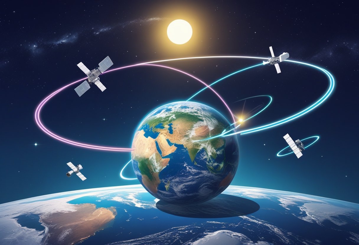
You rely on artificial satellites every day for navigation, communications, and weather data. GPS satellites orbit in medium Earth orbit with precise timing and known paths; your phone’s position fixes depend on those stable orbits and atomic-clock synchronization. Communication satellites in geostationary orbit remain fixed above the equator, letting broadcasters and satellite internet providers point antennas at a single spot. Remote sensing satellites in low Earth orbit image Earth for agriculture, disaster response, and environmental monitoring; their altitude and revisit time determine resolution and how often you get fresh imagery.

Operators plan launches and station-keeping burns to counter drag and keep orbital slots. Small errors accumulate from gravity irregularities and atmospheric drag, so routine adjustments preserve service quality. When you stream a map, check the weather, or call overseas, orbital mechanics keeps those signals on track.

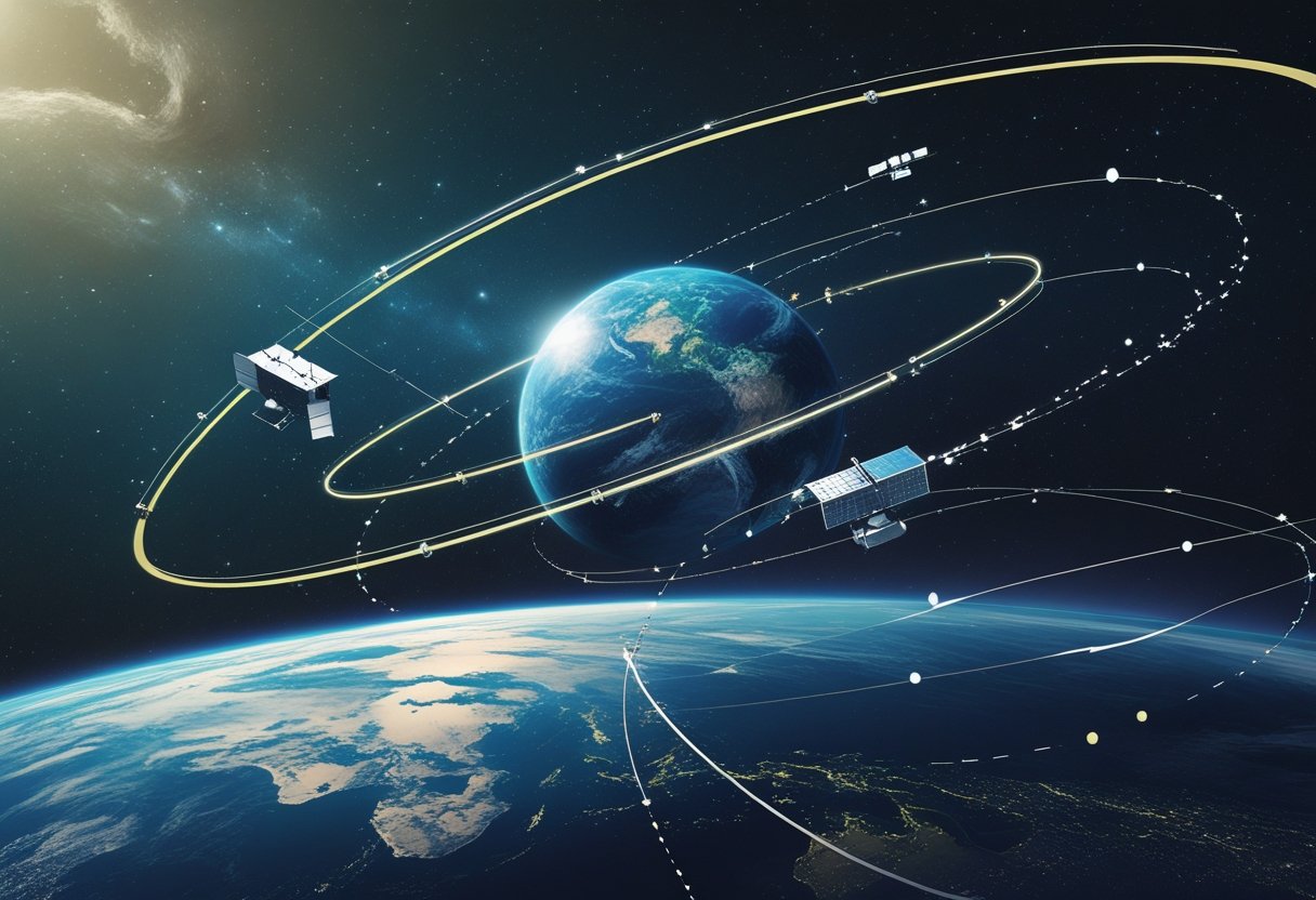
Orbit Determination and Tracking

Orbit determination uses observations of position and velocity to compute an object’s path under gravity. Ground radars, laser ranging, and telemetry from the spacecraft feed numerical models that include the gravitational constant, Earth’s nonuniform gravity field, and perturbations from the Sun and Moon. You can think of it as solving a moving-target puzzle: sensors supply snapshots, and the models interpolate the full trajectory.

Tracking networks update an orbit after maneuvers or atmospheric drag changes. Agencies maintain catalogs so satellite operators avoid collisions and plan rendezvous. If a satellite’s predicted path shifts, teams retarget ground stations and schedule correction burns. Accurate orbit determination keeps your satellite-based services precise and prevents close approaches that could create debris.

Challenges and Exciting Modern Uses

You face challenges like atmospheric drag, orbital debris, and perturbations from other bodies when operating satellites. Low Earth orbit satellites experience drag that lowers altitude and shortens mission life unless you perform periodic reboosts. Growing satellite constellations increase collision risk and require coordinated orbit management to prevent fragmenting events. Planetary orbits add complexity for missions to Mars: mission designers must time launches precisely to use gravity and minimal fuel.

Modern uses push orbital mechanics in new directions: large constellations for global broadband, hyperspectral remote sensing for precision agriculture, and smallsat swarms for rapid revisit imaging. You’ll also see gravity assists used to save fuel on interplanetary trips, and advanced orbit determination techniques—combining optical, radio, and GNSS data—improve navigation for autonomous spacecraft. These developments make orbital mechanics more operational and immediately useful to your phone, your farm, and your certainty that a probe will reach another planet.