You control a machine that finds its place among moving planets and invisible forces, and this article shows how that happens. Spacecraft navigation combines precise ground tracking, onboard sensors like star trackers and gyroscopes, and timed radio links so missions hit targets across millions of kilometers. You’ll learn how those systems work together to plan trajectories, determine position, and command course corrections.

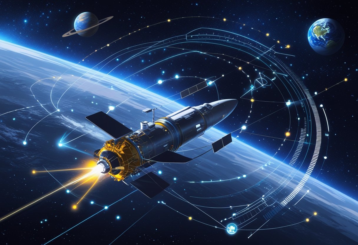
Expect clear explanations of how Earth-based tracking and antennas keep tabs on a craft, how onboard instruments keep it oriented, and how optical and autonomous methods cut communication delays. The post will also walk through orbit determination, trajectory maneuvers, and the practical challenges mission teams solve to turn navigation plans into successful missions.

Spacecraft Navigation Fundamentals

You will learn how precise math, physical laws, and planned paths keep a spacecraft on course. The next paragraphs explain the core ideas, how gravity and motion govern your craft, and how mission designers turn objectives into a usable reference trajectory.

Key Principles of Space Navigation

Spacecraft navigation centers on determining position, velocity, and orientation using measurements and models. You rely on observations (radio range, Doppler, optical star sightings) and onboard sensors (IMUs, star trackers) to update a state estimate that feeds guidance and control.

Navigation uses estimation algorithms such as the Kalman filter to fuse noisy measurements with predictive dynamics. You must model sensor bias, measurement noise, and external disturbances (solar radiation pressure, atmospheric drag near bodies). Accurate timing and synchronized clocks matter because a microsecond error maps to kilometers in deep-space range.

You also manage uncertainties through covariance analysis and covariance propagation. That tells you where to expect the spacecraft and how big correction burns should be. These principles let your mission design and astrodynamics teams set navigation performance requirements early.

Role of Orbital Mechanics

Orbital mechanics provides the governing equations you use to predict motion and design maneuvers. You work with Newtonian two-body dynamics as a baseline and add perturbations—third-body gravity, non-spherical gravity fields, and non-gravitational forces—when precision demands it.

You compute state propagation using numerical integrators (Runge–Kutta, multi-step) and linearize dynamics when performing sensitivity analysis or onboard guidance. Transfer design—Hohmann, bi-elliptic, patched-conic approximations—gives you low-energy routes; more complex missions use patched gravity assists or low-thrust trajectories that require continuous thrust modeling.

Mission planners express trajectories in orbital elements or Cartesian states and use astrodynamics tools to predict encounter geometries and relative motion. Understanding energy (specific orbital energy, Δv budgets) directly informs how much propellant and what navigation accuracy you need.

Reference Trajectory Design

A reference trajectory acts as the mission’s planned flight path and a target for navigation and guidance. You create it during mission design by specifying waypoints, timing constraints, and burn epochs to meet scientific or operational objectives.

Design tools optimize for fuel, time, or risk using objective functions and constraints. You include margin for maneuver execution errors, sensor outages, and modeling mismatches. The reference trajectory also defines coordinate frames and epochs for orbit determination and ground tracking.

During flight, the navigation team compares the propagated state to the reference trajectory to compute deviations and plan corrective maneuvers. You update the reference when major replans occur, but you generally keep the reference stable to provide predictable guidance and to simplify covariance budgeting.

Ground-Based Tracking and Communication

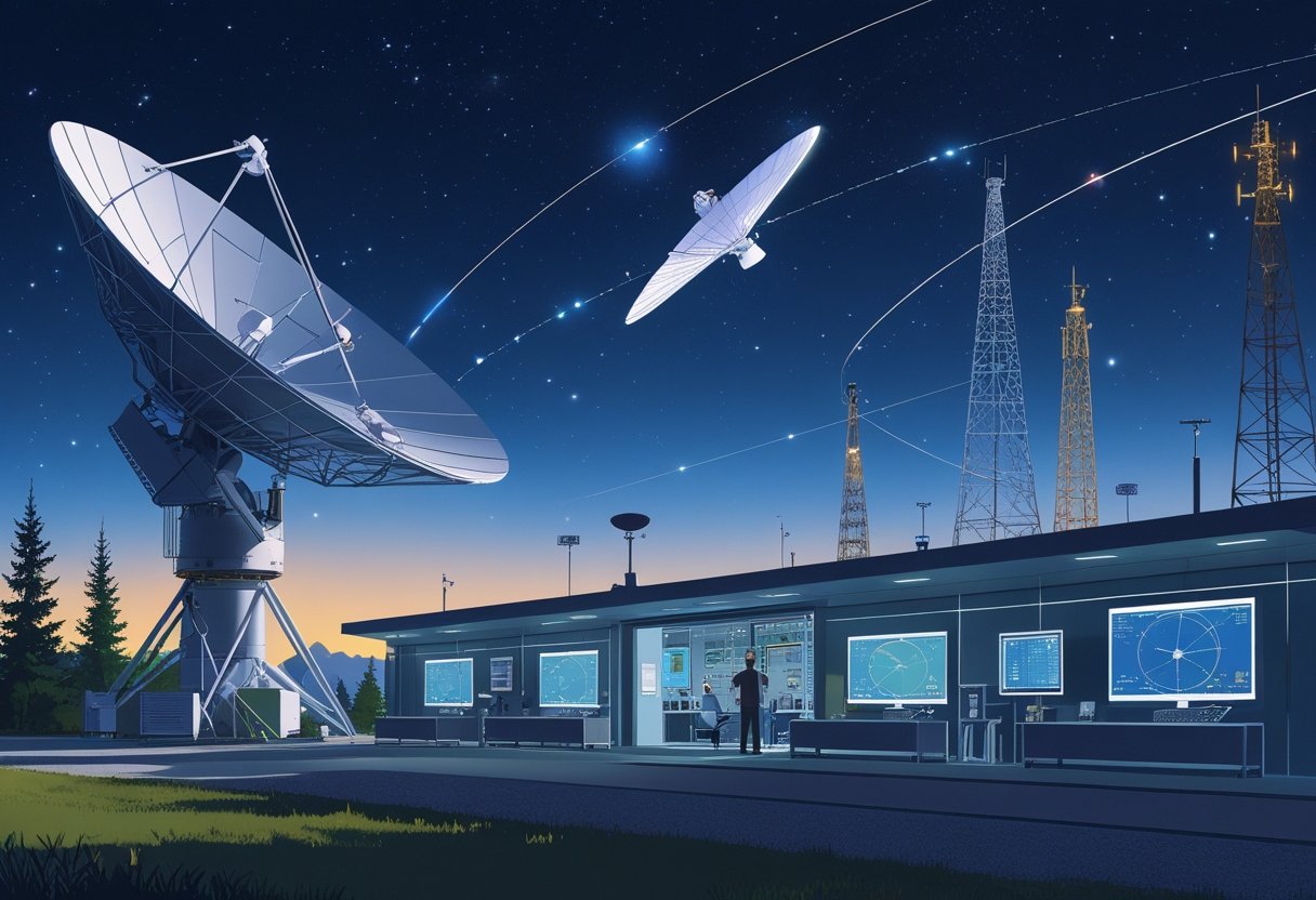
You rely on powerful ground systems to find, talk to, and measure a spacecraft’s position and motion across millions of kilometers. These systems use large dish antennas, precise timing, and signal-processing techniques to turn faint radio waves into position fixes, velocity data, and mission telemetry.

Deep Space Network and Ground Stations

You connect with spacecraft through networks of large dish antennas spread around the globe. NASA’s Deep Space Network (DSN) and similar facilities from ESA and other agencies operate 34–70 meter dishes that provide continuous visibility as Earth rotates.
Those antennas form an Earth-spanning triangle of listening posts; by scheduling handovers you keep a probe in contact nearly continuously during critical events.

Ground stations do more than receive signals. They transmit uplink commands, host high-stability reference clocks, and run data-processing centers that decode telemetry. You depend on site diversity and frequency allocation to mitigate weather, interference, and line-of-sight outages.

Radio Tracking Techniques

You determine spacecraft direction and motion using radio tracking methods such as angle measurement, doppler, and very long baseline interferometry (VLBI).
Large dish antennas measure the incoming signal’s angle in the sky; combining angle data from multiple stations yields triangulation-style fixes for lateral position.

VLBI uses synchronized observations from widely separated antennas to measure tiny phase differences, improving angular precision to milliarcseconds. Doppler tracking measures frequency shifts to derive radial velocity, while continuous carrier-phase tracking and telemetry modulation provide additional observables for orbit determination.

Ranging and Doppler Measurements

You measure distance with ranging and velocity with Doppler shifts. Two-way ranging sends a coded signal to the spacecraft and times the round-trip travel time to compute range precisely.
Range resolution depends on modulation bandwidth and timing precision; modern systems reach meter-level accuracy for near targets and kilometer-scale for deep-space probes.

Doppler tracking measures the fractional frequency shift of received carrier waves to infer spacecraft line-of-sight velocity. Combining periodic Doppler samples with range points yields trajectory estimates that feed flight-dynamics software. Both observables require nanosecond-level clock stability on the ground and careful calibration of station delays and media effects.

Communication Delays and Data Exchange

You must plan for light-time delays measured in seconds to hours. Round-trip travel time to Mars varies from several minutes to about 24 minutes; to the outer planets it can reach hours.
These delays force a store-and-forward approach: you uplink commands and wait for telemetry, or program autonomy onboard to execute time-critical actions.

Telemetry data travels on modulated radio carriers or optical links. Ground-based antennas decode telemetry frames, extract housekeeping and science packets, and forward them to mission control. You mitigate delay-related issues with predictive scheduling, on-board fault protection, and by using ground networks like the DSN or ESA stations to maximize contact windows and data throughput.

Onboard Navigation Systems and Instruments

These instruments give you continuous position, velocity, and attitude data without relying on Earth. They combine short-term inertial motion sensing with long-term celestial fixes and visual measurements to keep your spacecraft pointed and on trajectory.

Inertial Measurement Units and Inertial Navigation

You rely on an IMU (inertial measurement unit) as the spacecraft’s short-term dead-reckoning core. An IMU typically contains triads of accelerometers and gyroscopes that measure linear acceleration and angular rate about three axes. Integrating those signals in an inertial navigation system (INS) produces your computed velocity, position, and attitude between external updates.

High-performance gyros (fiber-optic or ring-laser) minimize drift; microelectromechanical (MEMS) units trade some precision for lower mass and power. You must calibrate biases and apply temperature compensation to prevent error growth. Extended Kalman filters usually fuse IMU outputs with star tracker or radio updates to constrain drift and keep navigation errors bounded.

Star Trackers and Celestial Navigation

Star trackers provide absolute attitude by imaging star fields and matching them to an onboard star catalog. You capture a camera frame, extract star centroids, and run a pattern-matching algorithm to identify the field. The tracker returns a quaternion or Euler angles with arcsecond-level accuracy for pointing and attitude control.

For longer-term position fixes, celestial navigation techniques—using angular measurements to known planets, moons, or pulsars—help correct INS drift. Modern approaches may also use X-ray pulsar timing for autonomous deep-space fixes. You depend on precise timekeeping and well-maintained star catalogs to transform star-tracker measurements into reliable spacecraft orientation and occasional position constraints.

Sun Sensors and Onboard Cameras

Sun sensors give simple, robust sun-line vectors for coarse attitude determination and safe-mode pointing. Most sensors are analog or photodiode arrays that report sun angle with degree-to-subdegree accuracy. You use them for initial acquisition after power-up and as cross-checks when star trackers are blinded by bright objects.

Onboard cameras serve multiple navigation roles: optical navigation during flybys, landmark-relative navigation for landings, and visual odometry near small bodies. You can measure apparent size, limb position, or feature tracks against star backgrounds to refine trajectory and attitude. Combining camera-derived measurements with IMU and star-tracker data in a navigation filter yields the precise, redundant solution you need for guidance and attitude control.

Optical and Autonomous Navigation Techniques

You will rely on visual measurements, onboard sensors, and autonomous filtering to estimate position and control flight paths precisely. These methods let your spacecraft use stars, planets, and pulsars as fixed references while onboard computers fuse measurements to correct trajectory and enable pinpoint landing.

Optical Navigation and Imaging

Optical navigation uses images from cameras to measure angles and apparent sizes of celestial objects. You capture star fields, moons, or target bodies with wide- or narrow-angle cameras and compare measurements to an onboard star catalog to determine attitude and line-of-sight directions.

Key steps:

• Acquire images and identify reference stars or landmarks.
• Measure bearing and apparent angular separation relative to catalog positions.
• Use triangulation and perspective (range-from-size or limb fitting) to estimate range and position.

Optical data integrates with inertial sensors to reduce drift. When approaching a body, real-time imaging refines the reference trajectory for descent and final targeting. For pinpoint landing, short-exposure images identify local landmarks and feed guidance updates into flight path control.

Pulsar Navigation and X-Ray Pulsars

Pulsar navigation treats certain pulsars as natural, stable clocks you can use for autonomous positioning. You measure pulse arrival times with an X-ray detector and compare them to predicted pulse schedules to compute your spacecraft’s position relative to the pulsar reference frame.

Why X-ray pulsars:

• X-rays penetrate background clutter and allow compact detectors.
• Pulse timing precision yields range errors of kilometers to sub-kilometer scale when multiple pulsars are used.

Operational flow:

• Select 3+ pulsars with well-characterized timing.
• Time-stamp pulses with an onboard clock and correct for spacecraft motion.
• Solve timing residuals to triangulate position.

This method reduces dependence on Earth-based ranging and supports deep-space autonomy, especially when combined with radiometric or optical updates.

Autonomous Navigation Algorithms

Autonomous navigation algorithms fuse sensor inputs and propagate a reference trajectory using probabilistic filters and model-based prediction. You run Extended or Unscented Kalman Filters (EKF/UKF) and batch least-squares on the onboard computer to estimate state (position, velocity, attitude) and update control commands.

Typical architecture:

• Sensors: star trackers, IMUs, cameras, X-ray pulsar detectors.
• Estimator: EKF/UKF for real-time updates; batch updates for orbit determination.
• Guidance: reference-trajectory follower that computes burn vectors and attitude maneuvers.

Algorithms also handle sensor dropouts and model uncertainties using fault detection and covariance inflation. For landing, the navigation stack supplies high-rate state updates to flight path control so you can perform trajectory corrections and achieve a pinpoint landing without continuous ground intervention.

Orbit Determination, Trajectory Corrections, and Maneuvers

You will learn how spacecraft locate themselves in space, how teams calculate needed course edits, and how those edits get executed using burns or thrusters. Expect specifics on position and velocity estimation, planning trajectory correction maneuvers (TCMs), and how delta-v budgets translate into real engine or thruster actions.

Orbit Determination Methods

Orbit determination reconstructs your spacecraft’s position and velocity from measurements you collect. Ground-based radiometric tracking (range and two-way Doppler) gives distance and line-of-sight velocity; very long baseline interferometry (VLBI) or angle tracking refines cross-track position. For near-Earth missions, GNSS receivers provide continuous position and velocity fixes.

You combine measurements in a dynamic model that includes gravity, atmospheric drag, solar radiation pressure, and known maneuvers. Kalman filters or batch least-squares estimators ingest telemetry and measurement noise characteristics to produce a best-fit state vector and covariance matrix. That covariance tells you navigation accuracy and informs whether a trajectory correction is needed.

Trajectory Correction Maneuvers

When your estimated state diverges from the mission reference trajectory, you plan a trajectory correction maneuver (TCM). You first compute the delta-V vector required to remove predicted dispersions at a critical future event, such as a planetary flyby or orbit insertion. Timing matters: an early small correction often costs less delta-v than a late large burn.

TCM planning uses target-pointing, conjunction constraints, and available propulsion performance. Deliverables include burn time, duration, attitude, and contingency windows. You simulate post-burn trajectories and update the orbit determination loop to confirm the TCM achieved the required accuracy. Multiple small TCMs in sequence reduce maneuver risk and improve final navigation accuracy.

Engine Burns, Thrusters, and Delta-V

You execute a TCM with either main engine burns or attitude-control thruster firings depending on required delta-v and precision. Main engine burns deliver large impulsive delta-v for transfers and orbit insertions. Reaction control system (RCS) thrusters provide smaller, pulse-mode firings for fine tune and stationkeeping.

Plan burns with burn-angle, thrust magnitude, and spacecraft mass to compute required duration: delta-v = thrust/mass × burn_time (integrated for variable thrust). You must account for plume impingement, engine minimum-thrust limits, and propellant margins. After each burn, you perform post-burn telemetry checks and an updated orbit determination to measure achieved delta-v and update future maneuver plans.

Mission Applications and Operational Challenges

You’ll learn how navigation requirements and risks change with orbit type, mission distance, and environmental forces. Expect specifics on positioning accuracy, common maneuvers, and the operational techniques teams use to keep spacecraft safe and on trajectory.

Low Earth Orbit, Geostationary, and Highly Elliptical Missions

In LEO you can often rely on GNSS for meter- to kilometer-level accuracy, so your satellite can do real-time attitude control, collision avoidance, and precise orbit determination with short latency. Operators typically schedule routine orbit determination passes and small delta-v maneuvers to maintain altitude and phase; drag and atmospheric density variations drive frequent station-keeping in low tens to hundreds of meters per day.

For GEO satellites, you maintain orbital slot within tight longitudinal bounds using periodic north-south and east-west station-keeping burns. GEO navigation depends on ground tracking and onboard sensors because GNSS reception is limited at geostationary distances. HEO missions face rapidly changing dynamics: perigee atmospheric drag and apogee radiation exposure require adaptive models and more frequent navigation updates.

Key operational concerns include space debris conjunction assessment in LEO, fuel budgeting for long station-keeping in GEO, and maintaining telemetry during HEO passes through variable radiation environments.

Interplanetary and Deep Space Navigation

When you move beyond cislunar space, GNSS becomes unreliable and navigation shifts to radiometric tracking and optical methods. Deep space navigation uses two-way Doppler and range from ground networks to reconstruct trajectories with typical uncertainties measured in kilometers for distant probes. You’ll use optical star-field or landmark-based measurements (image-based navigation) near small bodies to refine position to sub-kilometer levels during approach and landing.

Gravity assists provide powerful trajectory shaping but demand sub-kilometer targeting and precise timing at encounter to achieve the intended delta-v. Autonomous onboard navigation and predictive maneuvers reduce dependence on Earth when light-time delay grows to minutes or hours. Mission teams combine long-arc orbit determination with short-arc updates around critical events like orbit insertion or lander descent.

Impact of Gravitational Influences and Solar Radiation

Gravity from planets, moons, and non-uniform bodies perturbs your trajectory continuously. Accurate gravitational models — from spherical harmonics to mascon maps — become essential when you operate near irregular bodies or in low lunar orbit. Unmodeled gravity anomalies can shift orbits by kilometers over weeks if you don’t update state estimates and gravity fields.

Solar radiation pressure (SRP) acts like a tiny continuous thrust on large-surface-area spacecraft. You must model SRP using spacecraft cross-sectional area, optical properties, and attitude history to avoid meter- to kilometer-scale position errors over time. Combined gravitational and SRP effects demand frequent re-estimation of navigation models and occasional calibration burns to keep maneuver plans valid.

Overcoming Space Navigation Obstacles

You tackle navigation challenges with layered redundancy: combine GNSS, radiometric tracking, optical navigation, and inertial measurement for robust state estimation. Use Kalman filters and batch least-squares to fuse heterogeneous measurements and to quantify kilometer-level or better uncertainties when possible. During high-risk events, plan contingency maneuvers and carry fuel margins specifically for navigation correction.

Operational practices also matter: schedule regular orbit determination cycles, run conjunction assessments against debris catalogs, and update environmental inputs like atmospheric density and SRP coefficients. When GNSS signals are weak or absent, deploy autonomous navigation algorithms and pre-computed maneuver sequences to preserve mission objectives despite communication delays.